44 excel scatter diagram with labels
How to rotate axis labels in chart in Excel? 1. Go to the chart and right click its axis labels you will rotate, and select the Format Axis from the context menu. 2. In the Format Axis pane in the right, click the Size & Properties button, click the Text direction box, and specify one direction from the drop down list. See screen shot below: Improve your X Y Scatter Chart with custom data labels Select the x y scatter chart. Press Alt+F8 to view a list of macros available. Select "AddDataLabels". Press with left mouse button on "Run" button. Select the custom data labels you want to assign to your chart. Make sure you select as many cells as there are data points in your chart. Press with left mouse button on OK button. Back to top
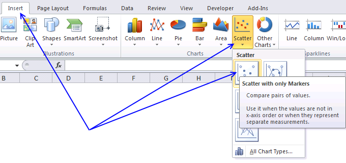
How to use a macro to add labels to data points in an xy scatter chart ... In Microsoft Office Excel 2007, follow these steps: Click the Insert tab, click Scatter in the Charts group, and then select a type. On the Design tab, click Move Chart in the Location group, click New sheet , and then click OK. Press ALT+F11 to start the Visual Basic Editor. On the Insert menu, click Module.
Excel scatter diagram with labels
How to Create a Sankey Diagram in Excel Spreadsheet Components of a Sankey Diagram in Excel. A Sankey is a minimalist diagram that consists of the following: Nodes: This is an element linked by “Flows.” Furthermore, it represents the events in each path. Flows: Flows link the nodes. And each flow is specified by the names of its source and target nodes in the “from” and “to” fields. Excel 2016 - Personalised labels for XY scatter plot In the Windows version (which I know best) there was the possibility to choose values for the labels that were not part of the XY plot itself but that option does not exist for the (2016) Mac version (at least I cannot find it). I can modify a few labels manually but with hundreds of point it is very complicated... Example: Label X Y a 1 2 b 3 4 Pie Chart in Excel | How to Create Pie Chart - EDUCBA If the labels are fewer, less we can compare easily with the other slices. If there are too many values, try using a column chart instead. Recommended Articles. This has been a guide to Pie Chart in Excel. Here we discuss how to create Pie Chart in Excel along with practical examples and a downloadable excel template.
Excel scatter diagram with labels. excel - How to label scatterplot points by name? - Stack Overflow I found this which DID work: This workaround is for Excel 2010 and 2007, it is best for a small number of chart data points. Click twice on a label to select it. Click in formula bar. Type = Use your mouse to click on a cell that contains the value you want to use. The formula bar changes to perhaps =Sheet1!$D$3 How to find, highlight and label a data point in Excel scatter plot Select the Data Labels box and choose where to position the label. By default, Excel shows one numeric value for the label, y value in our case. To display both x and y values, right-click the label, click Format Data Labels…, select the X Value and Y value boxes, and set the Separator of your choosing: Label the data point by name How to add conditional colouring to Scatterplots in Excel Step 3: Edit the colours. To edit the colours, select the chart -> Format -> Select Series A from the drop down on top left. In the format pane, select the fill and border colours for the marker. Repeat these steps for Series B and Series C. Here is our final scatterplot. How to plot a ternary diagram in Excel Feb 13, 2022 · Insert a Scatter Chart (XY diagram), e.g., ‘Scatter with Straight Lines’ (Figure 9) using the XY coordinates for the triangle from columns AA and AB. To make it into an equilateral triangle resize the chart area accordingly; for example 10 columns wide and 30 rows high, as in Figure 10.
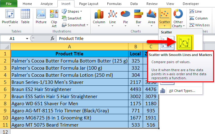
How to display text labels in the X-axis of scatter chart in Excel? Display text labels in X-axis of scatter chart Actually, there is no way that can display text labels in the X-axis of scatter chart in Excel, but we can create a line chart and make it look like a scatter chart. 1. Select the data you use, and click Insert > Insert Line & Area Chart > Line with Markers to select a line chart. See screenshot: 2. How to Create a Stem-and-Leaf Plot in Excel - Automate Excel To do that, right-click on any dot representing Series “Series 1” and choose “Add Data Labels.” Step #11: Customize data labels. Once there, get rid of the default labels and add the values from column Leaf (Column D) instead. Right-click on any data label and select “Format Data Labels.” When the task pane appears, follow a few ... Excel Scatter Chart with Labels - Super User Move the button down and out of the way of your data if you have more than a few columns. Paste your data in on top of the film data. Create scatter plots by selecting two column at a time and insert scatter (plot). Clicking on the button, which will add labels. Easy. How to Create Scatter Plots in Excel (In Easy Steps) To create a scatter plot with straight lines, execute the following steps. 1. Select the range A1:D22. 2. On the Insert tab, in the Charts group, click the Scatter symbol. 3. Click Scatter with Straight Lines. Note: also see the subtype Scatter with Smooth Lines. Note: we added a horizontal and vertical axis title.
Excel 2019/365: Scatter Plot with Labels - YouTube How to add labels to the points on a scatter plot. How to Make a Scatter Plot in Excel with Two Sets of Data? To get started with the Scatter Plot in Excel, follow the steps below: Open your Excel desktop application. Open the worksheet and click the Insert button to access the My Apps option. Click the My Apps button and click the See All button to view ChartExpo, among other add-ins. Select ChartExpo add-in and click the Insert button. Create an X Y Scatter Chart with Data Labels - YouTube How to create an X Y Scatter Chart with Data Label. There isn't a function to do it explicitly in Excel, but it can be done with a macro. The Microsoft Kno... Excel scatter chart using text name - Access-Excel.Tips Since Excel allows different chart types to be displayed in one chart, we are going to create a mix of bar chart (column chart) and scatter chart. Scatter chart is used to display the actual data point, while bar chart is to display Grade labels. - Create scatter chart for Range B20:C31 (Series 1)
Excel Scatter Chart - Super User
Scatter Plot In Excel - GeeksforGeeks In the Charts group, click Insert Scatter(X, Y) or Bubble Chart. Step 4: In the resulting menu, click Scatter. Once we have clicked that, our Scatter Plot will appear. Step 5: Now, to add label on x-axis and y-axis we have to click to the Design tab on the Ribbon. In the Chart Layouts group, click Quick Layout.
Find, label and highlight a certain data point in Excel scatter graph
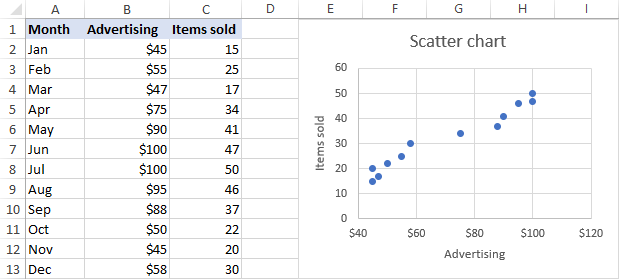
How to make a scatter plot in Excel - Ablebits How to create a scatter plot in Excel. With the source data correctly organized, making a scatter plot in Excel takes these two quick steps: Select two columns with numeric data, including the column headers. In our case, it is the range C1:D13. Do not select any other columns to avoid confusing Excel.
3d scatter plot for MS Excel
How to Create a Scatter Plot in Excel - Lifewire In Charts, select the Scatter (X,Y) or Bubble Chart drop-down menu. Select More Scatter Charts and choose a chart style. Select OK. Excel inserts the chart. Select the chart and make adjustments by clicking + (plus) to display elements you can apply or alter. This article explains how to create a scatter plot in Excel for Windows and Mac computers.
How to Make a Scatter Chart - ExcelNotes
How to Create Venn Diagram in Excel – Free Template Download First, let’s add data labels. Right-click on the data marker representing Series “Pepsi” and choose “Add Data Labels.” Step #15: Customize data labels. Replace the default values with the custom labels you previously designed. Right-click on any data label and choose “Format Data Labels.” Once the task pane pops up, do the following:
Daniel's XL Toolbox - Creating charts with labeled data clouds
The Problem With Labelling the Data Points in an Excel Scatter Chart Labelling the data points in an Excel chart is a useful way to see precise data about the values of the underlying data alongside the graph itself. In a column chart, for instance, you might show the value of the data point at the top of a column. A useful addition to a column chart is a set of data labels showing the value of each column.
Scatter Chart in Excel (Examples) | How To Create Scatter Chart in Excel?
How to Create Dot Plots in Excel? - EDUCBA In this article, we will see how we can create the dot chart in excel. Though we have conventional scatter plots added under Excel, those can not be considered as dot plots. Example of Dot Plots in Excel. Suppose we have month-wise sales values for four different years, 2016, 2017, 2018 and 2019, respectively.
Use a map in an Excel chart
Add labels to scatter graph - Excel 2007 - MrExcel Message Board Nov 10, 2008. #1. OK, so I have three columns, one is text and is a 'label' the other two are both figures. I want to do a scatter plot of the two data columns against each other - this is simple. However, I now want to add a data label to each point which reflects that of the first column - i.e. I don't simply want the numerical value or ...

How Do I Use Scatter Plots in Excel? (with Pictures) | eHow
Scatter Plot Chart in Excel (Examples) | How To Create Scatter ... - EDUCBA Step 1: Select the data. Step 2: Go to Insert > Chart > Scatter Chart > Click on the first chart. Step 3: This will create the scatter diagram. Step 4: Add the axis titles, increase the size of the bubble and Change the chart title as we have discussed in the above example. Step 5: We can add a trend line to it.
Making a scatter plot in Excel Mac 2011 - YouTube
How To Plot X Vs Y Data Points In Excel - Excelchat Figure 2 – Plotting in excel. Next, we will highlight our data and go to the Insert Tab. Figure 3 – X vs. Y graph in Excel . If we are using Excel 2010 or earlier, we may look for the Scatter group under the Insert Tab . In Excel 2013 and later, we will go to the Insert Tab; we will go to the Charts group and select the X and Y Scatter chart.

How to Make a Scatter Plot in Excel to Present Your Data
How To Create Scatter Chart in Excel? - EDUCBA To apply the scatter chart by using the above figure, follow the below-mentioned steps as follows. Step 1 - First, select the X and Y columns as shown below. Step 2 - Go to the Insert menu and select the Scatter Chart. Step 3 - Click on the down arrow so that we will get the list of scatter chart list which is shown below.
How to Make Scatter Plots in Microsoft Excel 2007
Scatter Graph - Overlapping Data Labels - Excel Help Forum We are not able to work with or manipulate a picture of one and nobody wants to have to recreate your data from scratch. 1. Make sure that your sample data are REPRESENTATIVE of your real data. The use of unrepresentative data is very frustrating and can lead to long delays in reaching a solution. 2.

Advanced Graphs Using Excel : create line plot with error bar plot in excel
Creating Scatter Plot with Marker Labels - Microsoft Community Right click any data point and click 'Add data labels and Excel will pick one of the columns you used to create the chart. Right click one of these data labels and click 'Format data labels' and in the context menu that pops up select 'Value from cells' and select the column of names and click OK.
Create a Scatter Diagram Using MS Excel 2007 - YouTube
Scatter Diagram Help | BPI Consulting - SPC for Excel A scatter diagram examines the relationship between two variables, X and Y. Quite often you are looking to determine if Y can be controlled by controlling X. This page shows to make a scatter diagram. The data can be downloaded here. This page contains the following: Data entry Creating a new scatter diagram Options for the scatter diagram Titles, Dates Labels Best fit equation Updating the ...

Scatter Chart in Microsoft Excel
Add Custom Labels to x-y Scatter plot in Excel Step 1: Select the Data, INSERT -> Recommended Charts -> Scatter chart (3 rd chart will be scatter chart) Let the plotted scatter chart be. Step 2: Click the + symbol and add data labels by clicking it as shown below. Step 3: Now we need to add the flavor names to the label. Now right click on the label and click format data labels.
How to improve the label placement for matplotlib scatter chart (code,algorithm,tips)? - Stack ...
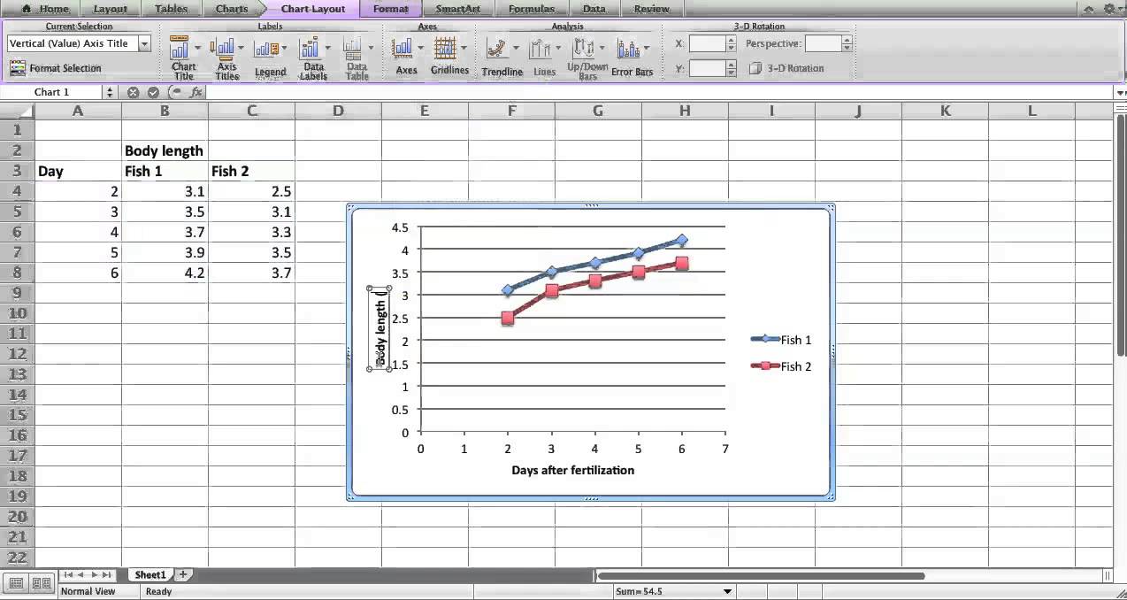
How To Add Axis Labels In Excel [Step-By-Step Tutorial] First off, you have to click the chart and click the plus (+) icon on the upper-right side. Then, check the tickbox for 'Axis Titles'. If you would only like to add a title/label for one axis (horizontal or vertical), click the right arrow beside 'Axis Titles' and select which axis you would like to add a title/label.
3d scatter plot for MS Excel
How to Add Labels to Scatterplot Points in Excel - Statology Step 3: Add Labels to Points. Next, click anywhere on the chart until a green plus (+) sign appears in the top right corner. Then click Data Labels, then click More Options…. In the Format Data Labels window that appears on the right of the screen, uncheck the box next to Y Value and check the box next to Value From Cells.

Excel: labels on a scatter chart, read from array - Stack Overflow
Pie Chart in Excel | How to Create Pie Chart - EDUCBA If the labels are fewer, less we can compare easily with the other slices. If there are too many values, try using a column chart instead. Recommended Articles. This has been a guide to Pie Chart in Excel. Here we discuss how to create Pie Chart in Excel along with practical examples and a downloadable excel template.
Scatter Plot with multiple series and filtering/sorting on values other than the series name : excel
Excel 2016 - Personalised labels for XY scatter plot In the Windows version (which I know best) there was the possibility to choose values for the labels that were not part of the XY plot itself but that option does not exist for the (2016) Mac version (at least I cannot find it). I can modify a few labels manually but with hundreds of point it is very complicated... Example: Label X Y a 1 2 b 3 4
Post a Comment for "44 excel scatter diagram with labels"